
![]()
Numerical simulation of quantum transport
Christoph Groth, Michael Wimmer, Anton Akhmerov, and Xavier Waintal
I will tell
- What is a scattering problem.
- What algorithms exist to solve it.
How to use Kwant to define and solve such problems (here we run some code).
- If you want to run code and don't have Kwant yet, get an account at http://cloud.sagemath.com/ now.
- Also please fill out the Kwant user survey at
http://kwant-project.org/2015-survey
The tight-binding scattering problem
Now to get conductance and other observables,
we only need to calculate $\Sigma_{\textrm{lead}}$, $G^R$, $G^<$, and we're done.
(that is what one mostly hears)
But there is a more intuitive definition.
The tight-binding scattering problem
has the Hamiltonian:
$$ H = \begin{pmatrix} \ddots & V_L\\ V_L^\dagger & H_{L}& V_{L}\\ & V_{L}^\dagger & H_L & V_L\\ & & V_L^\dagger &H_S\\ \end{pmatrix}, \quad \psi = \begin{pmatrix} \vdots \\ \psi_2 \\ \psi_1 \\ \psi_S \end{pmatrix} $$($H_L$ and $V_L$ are block-diagonal if there are many leads)
Modes in the leads
Since the leads are translationally invariant,
the lead wave function can be decomposed into eigenvectors of translation (lead modes)
the modes in the leads satisfy
$$ V_L \psi_0 + H \lambda \psi_0 + V_L^\dagger \lambda^2 \psi_0 = 0, $$or in a matrix form:
$$ \begin{pmatrix} -V_L^{-1} H_L & -V_L^{-1} \\ V_L^\dagger & 0 \end{pmatrix} \begin{pmatrix} \psi_0 \\ V_L^\dagger \psi_1 \end{pmatrix} = \lambda^{-1} \begin{pmatrix} \psi_0 \\ V_L^\dagger \psi_1 \end{pmatrix} $$...or in a more stable form (and reduced basis):
$ \tilde{H} = H_L + i AA^\dagger + i BB^\dagger,\quad V_L = A B^\dagger, \quad \tilde{\psi}_0 = B^+ \psi_0, \quad \tilde{\psi}_1 = A^+ \psi_1 $
Incoming and outgoing modes
Split all the eigenvectors into incoming, outgoing and evanecsent, such that:
$$\langle\psi_{\textrm{in}}|\hat{I}|\psi_{\textrm{in}}\rangle = 1$$$$\langle\psi_{\textrm{out}}|\hat{I}|\psi_{\textrm{out}}\rangle = -1$$$$\langle\psi_{\textrm{evan}}|\hat{I}|\psi_{\textrm{out}}\rangle = 0, \quad |\lambda_{\textrm{evan}}| < 1$$Finally, the equations to solve
Substituting the lead modes into Hamiltonian gives a linear system:
$$ \begin{split} \begin{pmatrix} - U_{\text{out}} & 1 \\ V_{L}^\dagger U_{\text{out}}\Lambda_{\text{out}} & H_\text{S} \end{pmatrix} \begin{pmatrix} \mathbf{S}\\ \psi_S \end{pmatrix} = \begin{pmatrix} U_{\text{in}}\\ -V_{\text{L}}^\dagger U_{\text{in}} \Lambda_{\text{in}} \end{pmatrix} \end{split}, $$with $U_{\text{in}}$ and $U_{\text{out}}$ wave functions of incoming and outgoing modes, and $\Lambda\equiv \textrm{diag}(\lambda_i)$.
From now on, we only need to write down these linear equations and solve them.
(NB: if we start by eliminating $\mathbf{S}$, the rhs becomes $H_S + \Sigma$)
Solving a linear system
Take a tight-binding system, assign #'s to sites, write down the matrix
kwant.plot(sys, ax=subplot(121, aspect='equal'), show=False)
h = sys.hamiltonian_submatrix().real
pyplot.spy(h, axes=subplot(122));

Naive solution
Perform gaussian elimination beginning to end:
pyplot.spy(h, axes=subplot(1, 2, 1))
p, l, u = scipy.linalg.lu(h)
pyplot.spy(l + u, axes=subplot(1, 2, 2));

Better idea (what most physicists would do)
Rearrange the sites into slices
(also known as recursive Green's functions)
pyplot.spy(h_rgf, axes=subplot(1, 2, 1))
p, l, u = scipy.linalg.lu(h_rgf)
pyplot.spy(l + u, axes=subplot(1, 2, 2));

What sparse linear algebra packages do
A hierarchic rearrangement (nested dissection)
pyplot.spy(h_diss, axes=subplot(1, 2, 1))
p, l, u = scipy.linalg.lu(h_diss)
pyplot.spy(l + u, axes=subplot(1, 2, 2));

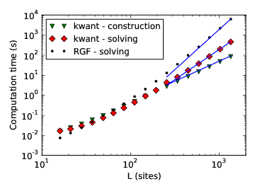
Algorithm of how to solve the scattering problem
- Construct a linear system of equations
(the one with lead modes) - Solve it efficiently
(so use a sparse linear algebra library)
Now let us solve some problems :-)

If you do not know python yet, you are missing a lot of fun.
Defining tight-binding systems (in kwant)
- There are many different tight binding systems
- There are only few sparse linear algebra libraries
- Libraries know of graphs, systems know of lattices, spins, superconductors, and many more.
So let's separate defining the system:
kwant.Builder
from solving it:
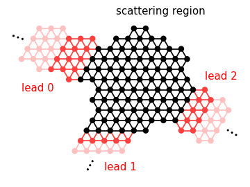
kwant.SystemAn example
Quantum Hall effect in a graphene with a quantum point contact
- Import the required packages
%matplotlib inline
from matplotlib import pyplot
import kwant
- Create the system and a lattice
hallbar = kwant.Builder()
graphene = kwant.lattice.general([[1, 0], [1/2, sqrt(3)/2]],  # Unit vectors
                                 [[0, 0], [0, 1/sqrt(3)]])  # Site positions
- Define the shape of the scattering region
def scattering_region(pos):
    x, y = pos
    return -50 < x < 50 and -30 < y < 30 and y**2 - x**2 < 14**2

hallbar[graphene.shape(scattering_region, (0, 0))] = 0.
Example (continued)
- Define the value of the hoppings (it depends on magnetic field and coordinates)
- Add the hoppings to the system
- Remove dangling bonds
def hopping(site1, site2, B=0.01):
    x1, y1 = site1.pos
    x2, y2 = site2.pos
    return -1 * exp(1j * B * (x1 - x2) * (y1 + y2))

hallbar[graphene.neighbors(1)] = hopping
# graphene.neighbors(2) for next-nearest neighbors

hallbar.eradicate_dangling()
Example (continued further)
- Repeat the same for the leads.
Leads are similar, only they have a translational symmetry
lead = kwant.Builder(kwant.TranslationalSymmetry((1, 0)))

def lead_shape(pos):
    return -30 < pos[1] < 30

lead[graphene.shape(lead_shape, (0, 0))] = 0.
lead[graphene.neighbors()] = hopping
- Attach the leads
hallbar.attach_lead(lead)
hallbar.attach_lead(lead.reversed());
Example (ready to solve)
- Check the result
kwant.plot(hallbar, site_size=1);

- Finalize the system
hallbar = hallbar.finalized()
Example (finally)
- Solve linear systems!
muvals = np.linspace(0.1, 0.4, 200)
conductances = [kwant.smatrix(hallbar, energy=mu).transmission(0, 1)
                for mu in muvals]
pyplot.plot(muvals, conductances);

Example: solve more
- calculate local density of states
ldos = kwant.solvers.default.ldos(hallbar, 0.20, args=[0.01])
kwant.plotter.map(hallbar, ldos, colorbar=False, cmap='gist_heat_r');

Exact diagonalization
- Find 6 eigenstates closest to Fermi level
h = hallbar.hamiltonian_submatrix(sparse=True).tocsc()
scipy.sparse.linalg.eigsh(h, sigma=0.1)[0]

Conclusions
- Quantum transport is as easy as defining and solving linear systems of equations.
- Defining tight such systems can be made easy.
- Solving them is also easy if using good libraries and clever algorithms.
Check Kwant out at http://kwant-project.org
More code examples:
- Basic stuff: http://downloads.kwant-project.org/examples/
- Topological stuff: http://topocondmat.org
- My favorite: http://arxiv.org/abs/1408.1563 (see ancillary files)
- For a reference:
Examples from research


Soft gap in Majorana wires (in preparation)
- What role does geometry of the nanowire experiment play?

- Different transverse modes in the wire have different flight times.

- Induced gap is inversely proportional to the flight time
- In ballistic samples the induced superconducting gap becomes soft: $\rho(E) \sim |E|$, for $|E| < \Delta_{\textrm{max}}$

- Disorder kills the trajectories with longest flight time first.
- There is a large range of disorder strengths, where the gap is soft and Majorana fermions are present

Thank you all.
The end.